Report: Social Media Content Classification
My research can be described in the broad area of social media content classification. For this semester, I focused on text classification. Text classification is basically an NLP problem. Popular NLP techniques include stemming, stop word elimination, sentiment analysis, and etc. A very popular algorithm often used in text analysis is topic modeling.
Topic Modeling
In machine learning and natural language processing, topic modeling is a type of statistical model for discovering the abstract “topics” that occur in a collection of documents. Latent Dirichlet Allocation (LDA) is a very popular algorithm to find the topic model of a collection of documents. David Blei and Andrew Ng’s pioneering paper on LDA makes two basic assumptions:
- There are a fixed number of patterns of word use, groups of terms that tend to occur together in documents. Call them topics.
- Each document in the corpus exhibits the topics to varying degree.
For example: we have some newspaper articles on soccer club games update and some narrations with fan-theories on DC and marvel comics. LDA will go through these and separate the documents based on the topics they discuss in those. LDA does not have any semantic knowledge of words. Rather it observes the words that are more likely to co-occur more statistically. While doing so, the algorithm finds some noise. Noise in LDA means finding patterns in co-occurrences of words that do not convey much useful information. For example, the words like articles, pronouns, negations, and etc. Removing such words is called stop word elimination. Another noise that often cause trouble to LDA topic modeling is that it might recognize “read”, “reads”, and “reading” as three different words. Hence, we can convert these words to their base form “read” and make LDA understand that these are all same words/topics. This step is called stemming.
Even after we go through topic modeling after fundamental preprocessing, it might be affected due to idioms that requires a collection of words to make a complete sense, or all documents might have repetitions of words for being from a specific domain that occurs so many times in these documents that they might not carry much information. In such case, we use TF-IDF that stands for term frequency-inverse document frequency. As the name suggests, it looks for the words that occur most in a document, however, it penalizes those words that not only occur more in a single document but occur in all documents. Kind of like the stop words, huh?
Topic modeling or TF-IDF cannot recognize synonyms. So, what should we do to teach our system to recognize the words that mean the same thing?
Word Embedding Models
Word embedding models are a modern approach of representing text in natural language processing (NLP). It is a way of representing a word in a dense vector space that is based on their meaning. It is an advancement on simple bag-of-words approach. Word embedding models are trained to be a fixed length dense and continuous valued vectors using a large corpus of text. Each word is represented by a point in the embedding space and these points are learned by moving around based on the words that usually surround that target word. In other words, a word is learned by the company it keeps that usually has “something” to do with the meanings of the words.
Let’s see a very popular example.
If we know a pair of words that are from same group like (man, king) and we want to get a similar pair where we know one entry like this: (woman, ?).
A standard word embedding model would suggest a like queen as the answer. Because it is the closest word that can replace king when woman replace the word man.
Something like this: queen = (king - man) + woman
Popular word embedding models include word2vec model by Google, GloVe by Stanford. There are some unconventional word embedding models available as well like urban dictionary model.
Download links for the pretrained models:
- GoogleNews word2vec model (Google Drive link)
- GloVe model (zip file)
- Urban Dictionary word2vec model
The model that you need to use depends on the application that you have in mind.
We can easily find already trained models for word2vec or Glove. However, you may need to develop/train the model from corpus at hand if you have a very specific application field in mind. For example, Google’s word2vec model was trained with entire Wikipedia corpus. The basic idea is similar to n-gram approach that means we need a group of words at a time to get idea of the context of the use of the word. Here, I show a general step through approach for training your word embedding model in Gensim, a more matured natural language processing framework than natural language toolkit (NLTK) that comes readily with python.
#assume we fit all our corpus in a variable in memory
sentences = 'This is a small corpora'
model = Word2Vec(sentences)

words = list(model.wv.vocab)	#vocabulary of the corpora
model.wv.save_word2vec_format('my_word_embedding_model', binary = True)
We can load a pretrained model by using:
model = Word2Vec.load('my_word_embedding_model')
If we have a group of words meaning similar thing and we know only one or two meaning the opposite, word embedding models can find the similar words; that can even specialized for our problem context if we chose to train our own word embedding models.
Up to this point I have talked about how we can use words or synonyms of words to perform natural language processing tasks. These sort of approaches work better with naive Bayes distribution model when the vocabulary for problem space is known and predefined. In case where we do not want our system to be limited by the EXACT words in the corpus rather we want to have an overall idea about the way of expression or conveying of information, we use sentiment analysis. Sentiment analysis being a popular technique comes readily with python NLTK library. Besides, a good number of resources can be found on the Internet about it. In this report, we will discuss a relatively new approach called tone analysis.
Tone Analysis with IBM Tone Analyzer
At first let’s ask the question, what is the benefit of using tone information instead of Sentiment information in text analysis or natural language processing?
There are several popular sentiment analysis tools out there like Vader sentiment analyzer, TextBlob, and etc. They each have their own way to represent the sentiment. For example, TextBlob sentiment analyzer gives a positive sentiment value and a negative sentiment value whereas Vader sentiment analyzer gives a positive, a negative, a neutral, and a compound (i.e. aggregated) sentiment score. All of these suggest the overall polarity of the sentiment. However, none of these has a way to distinguish among the positive emotions and negative emotions. For example, both sadness and anger are negative emotions, but there is an obvious distinction between them and they are often clearly distinguishable by human from written text. IBM Watson tone analyzer is a tool for estimating the emotional scores from text so that we can differentiate among emotions in negative sentiments and positive sentiments.
The IBM tone analyzer gives a sentence-wise score in a scale of 0 to 1 representing different aspects of the text. What do I mean with different aspects? This tool gives values of three aspects - emotions, language, and social - for any sentence supplied to it. Isn’t it fascinating? Huh! This tool is based on linguistic behavior and psychological theories.
The emotion score in the IBM Tone Analyzer represents the likelihood of a sentence to convey one of the following five emotions: anger, fear, disgust, joy, and sadness. These are a subset of the seminal classification of emotions by Ekman and Plutchik. The score is derived from a stacked ensemble framework. That means it combines predictions from many lower level models under a high level hood to achieve better performance. Examples of these low level features include: n-grams (unigrams, bigrams, and trigrams), punctuations, emoticons, curse words, greetings, and last but not the least sentiment polarity scores as we get from Vader or TextBlob. The high level hood uses a constrained optimization approach that is designed to handle co-occurrences of multiple emotions and noisy data. Thus, it becomes applicable for text we usually come across including on social media.
In the same way, language and social scores were calculated with analysis of learned features. Language scores evaluate three qualities in the words of a sentence: analytical, tentative, and confidence. As the names of the categories suggest, analytical scores represents the amount of reasoning and technical words in the sentences, tentative scores shows the amount of doubt in text, and confidence scores represent the degree of certainty in the text. In order to test the system’s performance, IBM tone analyzer used crowd-sourcing on a platform named CrowdFlower. The system achieved F1-score of ~0.7 with respect to experts’ annotations. The high F1-score means balanced performance of the system for different classes unlike accuracy which might get biased in case of unbalanced dataset.
The social scores indicate the likelihood of a sentence having the characteristics of the Big Five personality model: openness, conscientiousness, extroversion, emotional range, and agreeableness. Openness indicates the property of being open to new ideas; conscientiousness indicates the property of being methodical and organized; extroversion means the tendency of finding stimulation with others; emotional range (a.k.a. neuroticism) represents the extent to which emotion conveyed in the text shows sensitivity or stability; and lastly, agreeableness is the tendency of being compassionate.
So, an important question is: where can we use it? We can use this tool to analyze text where there is context involved. Well, those who advocate for n-grams can argue here that it is already done in their way. Let me give you an example.
Paragraph 1: It is a rainy day. Do I really need to out today?
Paragraph 2: It is a rainy day. School going kids are happy that their classes got canceled.
Paragraph 3: It is a rainy day. The humidity was very high and the large difference in atmospheric pressure flew the clouds towards the city causing the rain.
Now, tell me does n-gram on first sentence give you enough information about the context?
To know more about the IBM tone analyzer their official documentation is a good start. They got APIs in popular languages. And the best thing is, though it is a paid service, you get 3,000 API calls per month for free. That, I think, is enough for research purpose and for playing around with it.
Let’s get started by initializing tone analyzer.
from watson_developer_cloud import ToneAnalyzerV3
from watson_developer_cloud import WatsonApiException

tone_analyzer = ToneAnalyzerV3(
    version='timestamp',
    username='username',
    password='password',
    url='url'
)
Assuming we have all our documents as text entries in separate files, we can pass them to the tone analyzer.
def tone_analyze(fn, cls):
    try:
        with open(fn, 'r') as f:
            text = f.read()
        text = ''.join([i if ord(i) < 128 else ' ' for i in text])
        tone_analysis = tone_analyzer.tone(
            {'text': text},
            'application/json')
        # output = json.dumps(tone_analysis, indent=2)
        filename = fn[:-4]+'_output'+fn[-4:]
        json.dump(tone_analysis, open(filename, 'w'))
        pre_process(cls, filename)
    except WatsonApiException as ex:
        print "Method failed with status code " + str(ex.code) + ": " + ex.message
The above code snippet writes tone analysis result to a separate file named with _output suffix. We pass these files to be preprocessed. Here is the preprocessing code:
def pre_process(cls, filename):
    global columns
    output = json.load(open(filename))

    pprint(output.keys())

    # pprint(output['document_tone'])

    tone_names = ['Analytical', 'Confident', 'Tentative',
                'Anger', 'Joy', 'Sadness', 'Fear', 'Disgust',
                'Agreeableness', 'Conscientiousness', 'Emotion Range',
                'Extraversion', 'Openness']


    column_names = []
    for key in output.keys():
        for tone in tone_names:
            column_names.append(key+'_'+tone)
    column_names.append('sentences_count')
    column_names.append('class')
    print(len(column_names))
    columns = column_names
    print(columns)

    row = []

    for key in output.keys():
        if key=='document_tone':
            data = output['document_tone']['tones']
            # pprint(data)
            tone_dict = {}
            for entry in data:
                if entry['tone_name'] not in tone_dict.keys():
                    tone_dict[entry['tone_name']] = entry['score']
                else:
                    tone_dict[entry['tone_name']] += entry['score']
            for tone_name in tone_names:
                # print(tone_name)
                if tone_name in tone_dict.keys():
                    score = tone_dict[tone_name]
                else:
                    score = 0
                row.append(score)

        if key=='sentences_tone':
            tone_dict = {}
            for sentence_idx in range(len(output['sentences_tone'])):
                sentence = output['sentences_tone'][sentence_idx]
                data = sentence['tones']
                # pprint(data)
                for entry in data:
                    if entry['tone_name'] not in tone_dict.keys():
                        tone_dict[entry['tone_name']] = entry['score']
                    else:
                        tone_dict[entry['tone_name']] += entry['score']
            for tone_name in tone_names:
                # print(tone_name)
                if tone_name in tone_dict.keys():
                    score = tone_dict[tone_name]
                else:
                    score = 0
                row.append(score)
            row.append(len(output['sentences_tone']))
            row.append(cls)
    print(len(row))
    all_data.append(row)
In my research, I had text data of two different categories. I calculated the emotions, language, and social scores of those documents using IBM Tone Analyzer. I used these scores to see if there is any statistical differences among the scores of the documents of different classes using Student’s t-test.
Student t-test
Let me start by telling a story. There was a person named William Sealy Gosset. He worked at Guinness Brewery over one hundred years ago. He came up with a statistical test to show the difference between barley yield from two fields. When he wanted to publish the test, he was nervous, and instead of publishing it in his name, he used the pseudonym ‘Student’. To this day, this test is known as Student’s t-test instead of Gosset’s t-test.
What is t-test?
Imagine, you have two fields of same crops - field 1 and field 2. Maybe you want to compare the productions of these two fields with respect to a certain criteria. However, obviously it’s not wise to cut the crops from the whole fields for this. A test on samples from both these fields should be enough. Look at the following image:
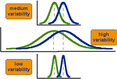
Image collected from: http://www.socialresearchmethods.net/kb/stat_t.htm
The top figure says that field 2 (indicated by blue line) has a higher mean than field 1 (indicated by green curve). But that just says a partial story. The fields can have different distributions as shown in the other two figures. Depending on that, the crops from these two fields can have statistical differences or not. And that’s where t-test becomes useful. We can see the t-value as a ratio between signal and noise. Signal means the numbers that can show the differences in two distributions, if any, and noise means the numbers that are just outliers. We can define signal as difference between group means and noise is the variability in the groups.
The formula that we are going to use:
\[t_{value} = \frac{\abs{field1_{mean} - field2_{mean}}}{\sqrt{\frac{field1_{var}}{field1_{count}} + \frac{field2_{var}}{field2_{count}}}}\]A sample calculation is shown here:
| field 1 | field 2 | |
|---|---|---|
| 15.2 | 15.9 | |
| 15.3 | 15.9 | |
| 16 | 15.2 | |
| 15.8 | 16.6 | |
| 15.6 | 15.2 | |
| 14.9 | 15.8 | |
| 15 | 15.8 | |
| 15.4 | 16.2 | |
| 15.6 | 15.6 | |
| 15.7 | 15.6 | |
| 15.5 | 15.8 | |
| 15.2 | 15.5 | |
| 15.5 | 15.5 | |
| 15.1 | 15.5 | |
| 15.3 | 14.9 | |
| 15 | 15.9 | |
| mean | 15.38125 | 15.68125 |
| standard deviation | 0.312449996 | 0.4069705149 |
| variance | 0.097625 | 0.165625 |
| count | 16 | 16 |
| t value calculated | 2.338821385 | |
| t value function | 0.02619805117 |
The t-value here is 2.3 that means there is more signal than noise.
If we had a null hypothesis: “There is no statistically significant difference between the samples.” That means any difference we find is just by chance. Hence, we need a critical value. If the our t-value is less than that we cannot reject the null hypothesis however if it is higher, we can reject the hypothesis and accept the alternative hypothesis.
Now, let’s look at the t-value table.
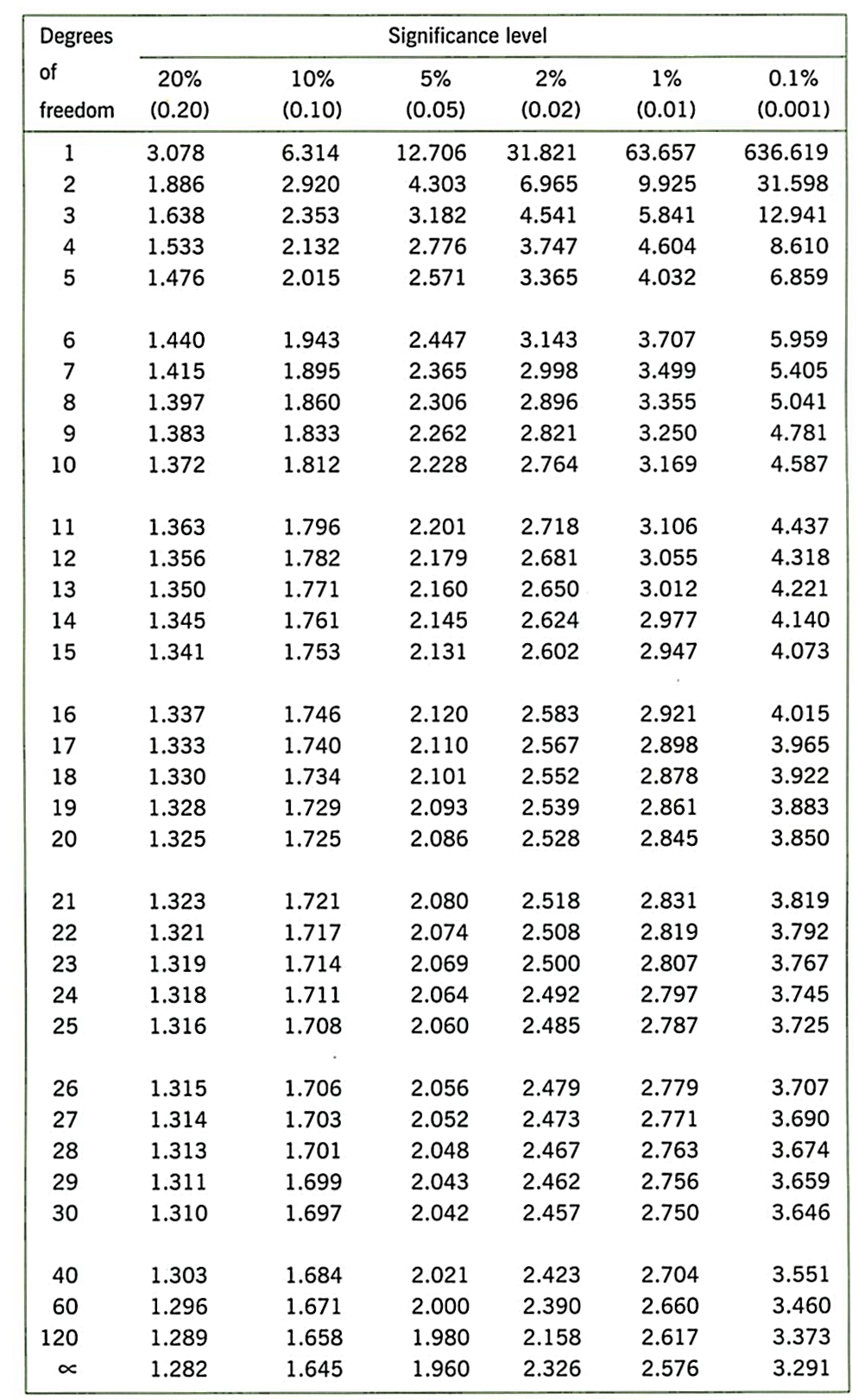
The degree of freedom is calculated as: df = count of samples from field 1 + count of samples from field 2 - 2 = 16 + 16 - 2 = 30 in our case. Generally, in inferential statistics, p = 0.05 is widely used. We are going to use that same value. Therefore, the critical value for us will be 2.042. Our t-value is greater than critical value, thus, we can reject the null hypothesis and accept the alternative hypothesis: There is statistically significant difference between the crops from two fields.
We can use the function: t-test as well to calculate the p value directly that gives us p = 0.026 < 0.05 and we can accept alternate hypothesis.
What if the calculated p value is greater than 0.05? There is no significant difference. What if it is slightly greater like 0.06? There is nothing like provisionally rejected in t-test. It just says you that you might try to apply that as a feature to machine learning algorithm on them to classify. It might be helpful however it will not be decisive.